Navigate this blog
In this post
How Do Machines Think and Learn?
In my previous blog, Before the AI Boom: A Look Back in Time!, we explored some of the ideas that shaped Artificial Intelligence and the questions that continue to fascinate us about machine intelligence.
One question that came up was about the learning aspects of a machine: At what point can we say that a machine can independently learn without human guidance?
Before we explore that question, let’s start with the basics.
What Does It Mean for a Machine to Learn?
Tom Mitchell, in his 1997 book Machine Learning, provided a classic definition of Machine Learning:
A computer program is said to learn from experience E with respect to some class of tasks T and performance measure P, if its performance at tasks in T, as measured by P, improves with experience E.
In simple terms, a machine is said to learn when its performance on a task improves through experience.
This is the classic definition, and there are many other ways to describe Machine Learning. However, the question still remains: What exactly is happening when a machine learns?
Let’s explore this through two classical problems in supervised Machine Learning:
- Classification
- Regression
1. Classification: Linear or Non-Linear?
Classification is about predicting a class label. For example, imagine that we have a dataset containing red and blue data points, and we want a machine to classify each point as either red or blue.
Let’s start small.
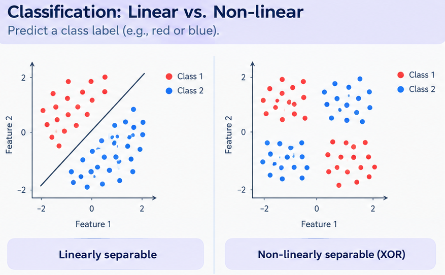
Image 1: Two classification problems, one where red and blue points can be separated by a straight line, and another illustrating the classic XOR problem. (Note: This image was generated with the help of ChatGPT.)
The Linearly Separable Case
If the data points can be separated by a straight line, we say that the problem is linearly separable.
Suppose we provide the machine with a labelled dataset containing spatial coordinates and their corresponding class labels, “red” or “blue”.
The machine analyses the data points and learns a decision boundary that separates the two classes. In a two-dimensional space, this boundary can be represented by a straight-line equation.
This is where we can begin to understand what we might informally call the machine’s thinking process. The machine uses the available data to identify patterns and construct a mathematical representation that can help it predict the class of a new data point.
But what is the machine learning?
During training, the model adjusts its parameters to find a decision boundary that performs well on the labelled data. Depending on the algorithm, the objective may be to minimise classification error, optimise a loss function, or maximise the margin between classes.
For example, Logistic Regression can learn a linear decision boundary, while a Support Vector Machine (SVM) can learn a boundary that maximises the margin between classes.
The important distinction is that the machine is not simply memorising the coordinates of every red and blue point. It is learning a representation that can be used to classify previously unseen points.
The Non-Linearly Separable Case
What happens when the data points cannot be separated by a straight line?
Consider the classic XOR problem, where points belonging to the same class occupy diagonally opposite regions of the coordinate space. A single straight line cannot correctly separate both classes.
This is a non-linearly separable classification problem.
Here, we need a more flexible decision boundary. Depending on the problem, a model might use a curved boundary, a higher-dimensional representation, or a combination of transformations to distinguish between the classes.
For example, an SVM with a suitable non-linear kernel can learn a non-linear decision boundary.
We can extend this idea beyond two classes as well. Real-world classification problems involving images, videos, and text can require much more complex representations than a straight line.
The underlying idea, however, remains the same: the model uses data to learn a representation that helps it predict the appropriate class.
2. Predict, Compare, Learn: The Neural Network Perspective
When we move from classical Machine Learning to neural networks, the process becomes particularly interesting.
François Chollet describes the neural network training process through a simple cycle:
Predict → Compare → Learn
Let’s understand what happens in each step.
1. Predict
The machine receives an input and uses its current model parameters to produce a prediction.
For a classification problem, the output might be the predicted class or the probabilities associated with different classes.
At this point, the model is applying what it has learned so far. Its prediction may be correct or incorrect.
2. Compare
During supervised training, the prediction is compared with the expected output, or ground-truth label.
A loss function measures how far the prediction is from the desired result. The loss provides a numerical signal that helps the model determine how well it is performing.
3. Learn
The model uses this signal to adjust its parameters in an attempt to reduce the loss.
In a neural network, these parameters are primarily the weights and biases. Training algorithms such as gradient descent, typically combined with backpropagation, help determine how the parameters should be updated.
The process repeats across training examples and iterations.
Over time, the model may learn parameters that allow it to make more accurate predictions on new data.
This brings us back to our original question.
Is the machine thinking when it makes a prediction, or is it learning when it changes its parameters?
For the purpose of this discussion, we can use thinking as an analogy for analysing inputs and generating predictions, and learning for the process of adjusting the model based on experience and feedback.
The distinction is useful, but we must remember that it is an explanatory analogy rather than a formal division in Machine Learning.
3. Regression: Predicting a Value
Classification predicts a class label. Regression, on the other hand, predicts a continuous value.
For example, we might want to predict a house price based on its area, location, and other characteristics. These input variables are commonly called predictors or features.
Let’s simplify the problem and consider data points described by a predictor (x) and a corresponding target value (y).
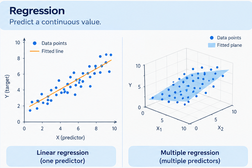
Image 2: A linear regression example showing data points and a fitted line, alongside a multiple regression example with several predictors. (Note: This image was generated with the help of ChatGPT.)
Given a set of data points, we want to fit a line that captures the relationship between the predictor and the target value.
The machine analyses the data and estimates the parameters of a line that fits the observed points according to a chosen objective. In ordinary least-squares linear regression, for example, the model minimises the sum of the squared differences between the observed values and the values predicted by the line.
Once again, we can use the idea of thinking to describe the process of representing the relationship between the input and the target.
The machine is not necessarily finding a line that passes through every point. Real-world data often contains noise, variation, and relationships that cannot be represented perfectly by a straight line.
Instead, the model learns a relationship that aims to make useful predictions.
For example, in a simple linear regression model, the parameters include the slope and intercept of the line.
When we have multiple predictors, we move to multiple regression. The model estimates how the target variable relates to several input variables, while accounting for the form of the model being used.
The objective remains to learn a relationship that performs well according to the chosen loss function and evaluation criteria.
4. Parameters, Hyperparameters, and Learning
Throughout these examples, we have encountered parameters that change during training.
In linear regression, these may be the slope and intercept. In a neural network, they include the weights and biases connecting the different layers.
These are model parameters—the values the training process adjusts to improve the model’s predictions.
We also have hyperparameters, which influence how the model is configured or how training takes place.
For example, the learning rate controls the size of parameter updates during gradient-based optimisation. The choice of kernel in an SVM determines the form of the similarity function used by the model.
Unlike model parameters, hyperparameters are generally set before training or selected through a separate tuning process.
Both matter, but they play different roles.
So, Can Machines Think? Can They Learn?
Let’s return to the questions that started this discussion.
Can machines think?
We have built systems that analyse inputs, identify patterns, construct representations, and produce predictions or decisions. We can use thinking as a way to describe these computational processes, as long as we do not automatically equate them with human thought or conscious experience.
Can machines learn?
Yes. Machine Learning systems can improve their performance on a task by adjusting their model parameters using data, feedback, or other forms of experience. The precise learning process depends on the algorithm and the learning approach.
But does learning always require human guidance? Not necessarily. Some systems learn from labelled examples, while others learn through unlabelled data, interaction with an environment, or feedback generated by the system itself. Human involvement can vary considerably.
Perhaps the more useful question is not simply whether machines can think or learn, but what kind of thinking-like computation are we observing, what exactly is the machine learning, and how do we know that it is improving?
Understanding these distinctions gives us a better starting point for exploring the capabilities and limitations of Machine Learning.